Effective Visualization of Multi-Dimension Image Data in Python

Multi-dimensional image data is, generally speaking, cumbersome to visualize.

In scientific imaging (or in most imaging areas), multi-dimensional images are very common. The additional dimension could be anything from the physical 3rd dimension ("Z axis"), where 2D images are taken at different depths; to the time dimension, where 2D images are taken at different time intervals; to different channels in scientific imaging instruments such as atomic force microscopes or in RGB images.

We will use seaborn-image, an open source image visualization library in Python based on matplotlib.

It is heavily inspired by the popular seaborn library for statistical visualization

Installation

pip install -U seaborn-image

You can find out more about the seaborn-image project on GitHub.

Load sample 3D data

import seaborn_image as isns

cells = isns.load_image("cells")
cells.shape

(256, 256, 60)

Visualize

We will use ImageGrid from seaborn_image to visualize the data. It will plot a series of images on a grid.

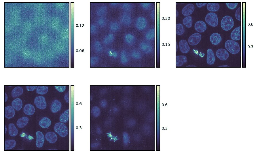
To begin, we will only plot a few selected slices using the slices keyword argument.

g = isns.ImageGrid(cells, slices=[10, 20, 30, 40, 50])

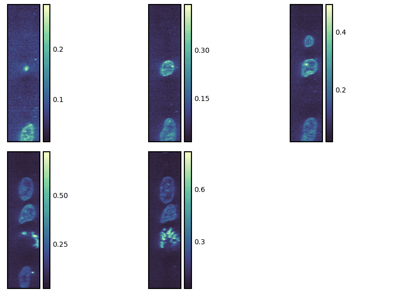
By default, the slices are taken along the last axis. However, we can take them along another dimension using the axis keyword argument.

g = isns.ImageGrid(cells, slices=[10, 20, 30, 40, 50], axis=0)

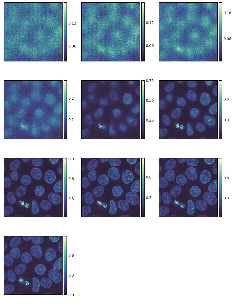
We can also specify different start/stop points as well as step sizes to take using the start, stop and step parameters, respectively.

In the code below, we are starting with the 10th slice and going up to the 40th slice with steps of 3.

The slices and steps are taken over the last axis if not specified.

g = isns.ImageGrid(cells, start=10, stop=40, step=3)

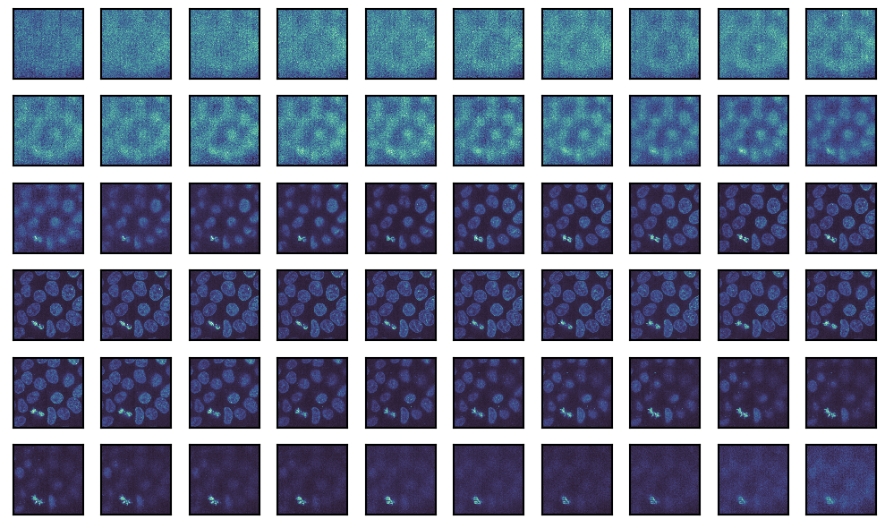
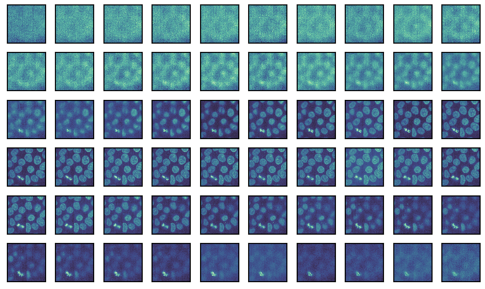
We can also just plot all the images without any indexing or slicing.

g = isns.ImageGrid(cells, cbar=False, height=1, col_wrap=10)

Note - We altered the height of the individual images and the number of image columns.

Transformations

Finally, we can also apply transformations to the image and visualize it. Here, we will adjust the exposure using the adjust_gamma function from scikit-image.

We can achieve this by passing the function object to the map_func parameter. Additional parameters to the function object can be passed as keyword arguments.

from skimage import exposure

g = isns.ImageGrid(
    cells,
    map_func=exposure.adjust_gamma,  # function to map
    gamma=0.5,  # additional keyword for `adjust_gamma`
    cbar=False,
    height=1,
    col_wrap=10)

ImageGrid returns a seaborn_image.ImageGrid object and is a figure-level function, i.e. it generates a new matplotlib figure. We can access the figure and all the individual axes using the fig and axes attributes, respectively. This means that for any customizations that are not directly available in seaborn-image (see documentation), we can drop down to matplotlib and use its powerful API.

Overall, as we have seen throughout this post, seaborn-image allows us to be more productive by providing a high-level API for quick, effective and attractive image data visualization.

You can find out more about the seaborn-image project on GitHub.

Thanks for reading!